2-nuclides plots

Introduction

How to use this document?

This html page is derived from an R Markdown Notebook. You can copy/paste the various lines of code into your own R script and run it in any R session.

Objectives

The objective of this notbook is to explore the construction of 2-nuclides plots.

Set up

The first thing we have to do is to load the TCNtools library (once it has been installed)

library("TCNtools")

We should the define the basic parameters we are going to use for the computation, which are two vectors :

a vector with the attenuation lengths for different particules (in g/cm\(^2\))
- neutrons for spallation reactions \(\Lambda_{spal}\)
- stopping muons \(\Lambda_{stop}\)
- fast muons \(\Lambda_{fast}\)
a matrix with the SLHL production rates (in at/g/a), in this case for the st scaling scheme (Stone (2000)), and decay constant \(\lambda\) (in a\(^{-1}\)) for the nuclides of interest.

We can first load the attenuation length data (g/cm\(^2\)). Documentation of this dataset is accessible with ?Lambda.

data(Lambda) # we load a vector containing the attenuation length into the environment
print(Lambda)

## Lspal Lstop Lfast 
##   160  1500  4320

rho = 2.7 # we also define the density (g/cm3)

The the production and decay parameters. Documentation of this dataset is accessible with ?prm.

data(prm) # we load a matrix containing the production/decay parameters into the environment
print(prm)

##               Be10         Al26          C14
## Pspal  4.01000e+00 2.793000e+01 1.224000e+01
## Pstop  1.20000e-02 8.400000e-01 3.310000e+00
## Pfast  3.90000e-02 8.100000e-02 0.000000e+00
## lambda 5.09667e-07 9.667325e-07 1.209681e-04

We also need to define the properties of our site of interest and compute the relevant scaling parameters.

altitude = 1000 # elevation in m
latitude = 45 # latitude in degrees
P = atm_pressure(alt=altitude,model="stone2000") # compute atmospheric pressure at site
S = scaling_st(P,latitude) # compute the scaling parameters according to Stone (2000)

We also need to define the properties of our site of interest and compute the relevant scaling parameters. This is a first approximation which consider that all samples are close and have similar positions. We will see later how to deal with situations where samples have different positions and hence different scaling parameters.

altitude = 1000 # elevation in m
latitude = 45 # latitude in degrees
P = atm_pressure(alt=altitude,model="stone2000") # compute atmospheric pressure at site
st = scaling_st(P,latitude) # compute the scaling parameters according to Stone (2000)

Steady-state denudation and constant exposure curves

Two-nuclides plots are usually build around two curves representing the predictions, in terms of concentrations, for end-member simplified situations :

steady-state denudation, where the concentrations of the nuclides of interest are computed for various values of surface denudation rates
constant exposure, where the concentrations of the nuclides of interest are computed for various duration of surface exposition, with no denudation

We will use the Eulerian point of view (function solv_conc_eul) to compute the concentrations, which is done by function tnp_curves.

In order to avoid messing up things later we define here once and for all which is nuclide 1 and which is nuclide 2, according to their respective \(\tau_{1/2}\) :

N1 = "Be10" # longer half-life
N2 = "Al26" # shorter half-life

We compute the data for these two curves.

tmp = tnp_curves(prm[,N1],prm[,N2],Lambda,st,rho)
ss_ero = tmp[[1]]
cst_exp = tmp[[2]]

The default parameters for the ranges of denudation rates and exposure ages can be adjusted is needed.

Now that we can plot everything in a two-nuclide graph. While not mandatory, it is recommended to organize the plot this way :

X-axis : longer half-life nuclide (our \(N_1\))
Y-axis : ratio of shorter to longer half-life nuclides (our \(N_2/N_1\))

plot(NA,xlim=range(cst_exp$C1,ss_ero$C1),ylim=range(cst_exp$C2/cst_exp$C1,ss_ero$C2/ss_ero$C1),log="x",
     xlab=paste(N1,"(at/g)"),ylab=paste(N2,"/",N1))
lines(cst_exp$C1,cst_exp$C2/cst_exp$C1,lty=2,col="khaki4") # constant exposure, dashed line
lines(ss_ero$C1,ss_ero$C2/ss_ero$C1,col="khaki4") # steady-state erosion, solid line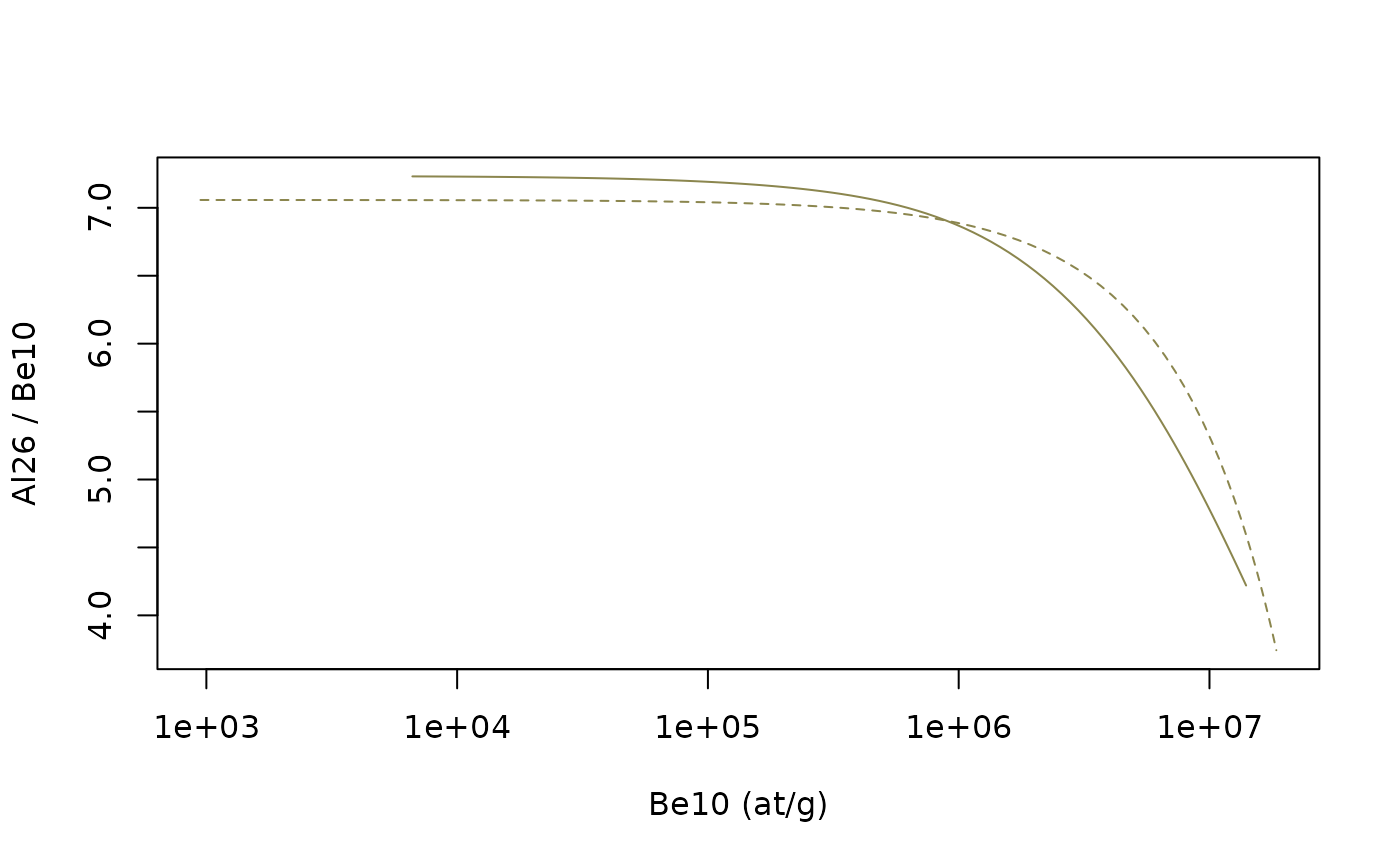

The extent of the plot can be modified to correspond more closely to the reported data.

Adding data

We are now going to add some data points. Here is a data set.

data = data.frame(
  Be10=c(1176054,1798477,4436623,759349,9045913),
  Be10_e=c(23955,44533,70831,16776,132287),
  Al26=c(7269896,11588554,24975976,4867323,43197465),
  Al26_e=c(235842,351978,429957,149041,715748),
  lat=c(30.1,33,32.2,30.4,32.7),
  alt=c(1000,900,1200,1100,960),
  name=c(1,2,3,4,5))
  colnames(data) <- sub(N1, "N1", colnames(data)) # we just change the column names to have everything in terms of N1 and N2
  colnames(data) <- sub(N2, "N2", colnames(data)) 
  print(data)

##        N1   N1_e       N2   N2_e  lat  alt name
## 1 1176054  23955  7269896 235842 30.1 1000    1
## 2 1798477  44533 11588554 351978 33.0  900    2
## 3 4436623  70831 24975976 429957 32.2 1200    3
## 4  759349  16776  4867323 149041 30.4 1100    4
## 5 9045913 132287 43197465 715748 32.7  960    5

In a first time we are going to compute average scaling parameters for the whole dataset, and we will see later how to account for the differences in locations between the samples.

  data$P = atm_pressure(alt=data$alt,model="stone2000") # compute atmospheric pressure at each site
  data = cbind(data,scaling_st(data$P,data$lat)) # compute the scaling parameters according to Stone (2000), and merge with samples table
  S = c(mean(data$Nneutrons),mean(data$Nmuons)) # average of the st scaling parameters

Simply plotting data points

We recompute the reference curves for the sample scalings

tmp = tnp_curves(prm[,N1],prm[,N2],Lambda,S,rho)
ss_ero = tmp[[1]]
cst_exp = tmp[[2]]

Then we plot everything.

plot(NA,xlim=range(data$N1),ylim=range(data$N2/data$N1),log="x",
     xlab=paste(N1,"(at/g)"),ylab=paste(N2,"/",N1))
lines(cst_exp$C1,cst_exp$C2/cst_exp$C1,lty=2,col="khaki4") # constant exposure, dashed line
lines(ss_ero$C1,ss_ero$C2/ss_ero$C1,col="khaki4") # steady-state erosion, solid line
#
points(data$N1,data$N2/data$N1,pch=21,bg="white",cex=2) 
text(data$N1,data$N2/data$N1,data$name,cex=0.9)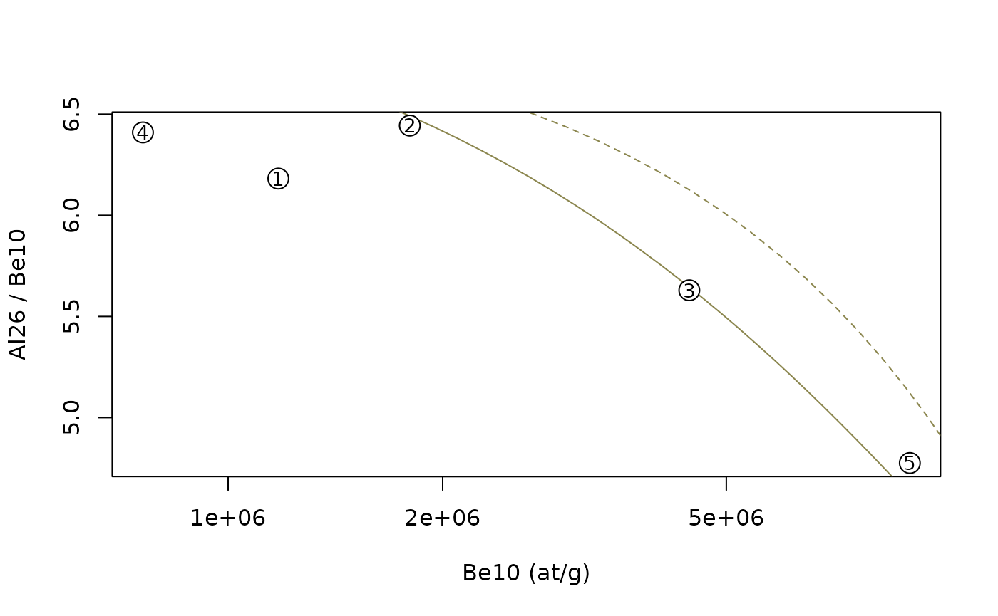

Dealing with uncertainties

We are now going to plot the uncertainties associated with each measurement. Is important to note that X (N1) and Y (N2/N1) are correlated, which implies that we can not simply display uncertainty as error bars. The function tnp_ellipse allows to compute an error ellipse accounting for this correlation. This function takes the concentration and their uncertainties as well as desired confidence level, and return the contours of the corresponding ellipses.

plot(NA,xlim=range(data$N1),ylim=range(data$N2/data$N1,4.5,7),log="x",
     xlab=paste(N1,"(at/g)"),ylab=paste(N2,"/",N1))
lines(cst_exp$C1,cst_exp$C2/cst_exp$C1,lty=2,col="khaki4") # constant exposure, dashed line
lines(ss_ero$C1,ss_ero$C2/ss_ero$C1,col="khaki4") # steady-state erosion, solid line
#
el = tnp_ellipse(data$N1, data$N1_e, data$N2, data$N2_e,confidence=0.68)
for (i in 1:length(el)) {polygon(el[[i]],col="pink",border="grey")}
text(data$N1,data$N2/data$N1,data$name,cex=0.8)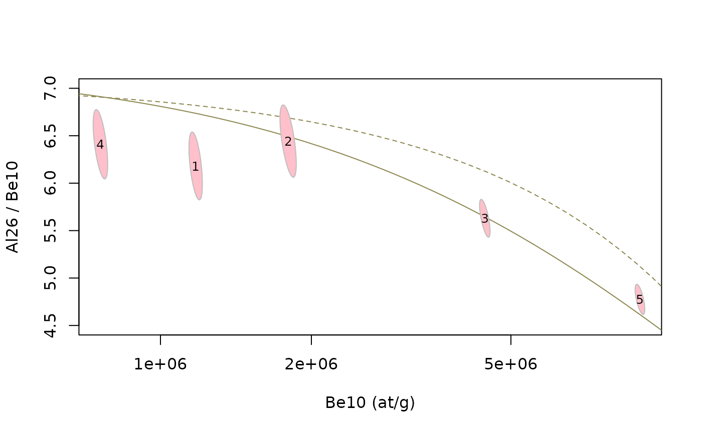

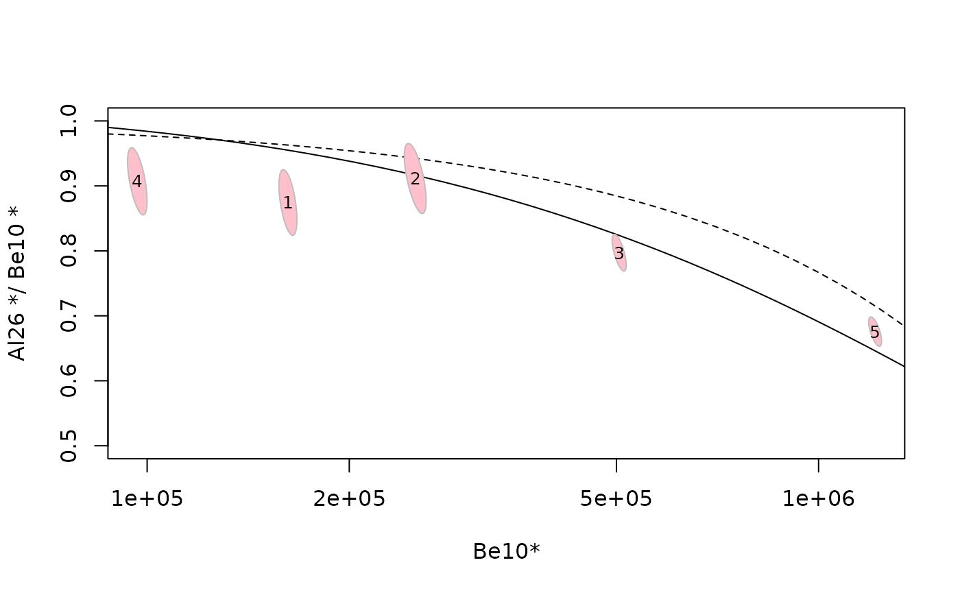
Normalizing

In some cases the various samples that we want to plot on a two-nuclides graph might have different spatial origins, with very different latitude, longitude and elevation, and therefore different scaling factors. In this case we need to normalize both the sample data and the steady-state denudation and constant exposure curves.

Each concentration is normalized by the SLHL production rate.

tmp = tnp_curves(prm[,N1],prm[,N2],Lambda,c(1,1),rho)
ss_ero_n = tmp[[1]]
cst_exp_n = tmp[[2]]
ss_ero_n$C1 = ss_ero_n$C1/sum(prm[1:3,N1])
ss_ero_n$C2 = ss_ero_n$C2/sum(prm[1:3,N2])
cst_exp_n$C1 = cst_exp_n$C1/sum(prm[1:3,N1])
cst_exp_n$C2 = cst_exp_n$C2/sum(prm[1:3,N2])

We also normalize the data (by the local surface production rate),

data$N1n   = data$N1   / (prm[1,N1]*data$Nneutrons + prm[2,N1]*data$Nmuons + prm[3,N1]*data$Nmuons)
data$N1n_e = data$N1_e / (prm[1,N1]*data$Nneutrons + prm[2,N1]*data$Nmuons + prm[3,N1]*data$Nmuons)
data$N2n   = data$N2   / (prm[1,N2]*data$Nneutrons + prm[2,N2]*data$Nmuons + prm[3,N2]*data$Nmuons)
data$N2n_e = data$N2_e / (prm[1,N2]*data$Nneutrons + prm[2,N2]*data$Nmuons + prm[3,N2]*data$Nmuons)

And finally plot,

plot(NA,xlim=range(data$N1n),ylim=range(data$N2n/data$N1n,0.5,1),log="x",
     xlab=paste(N1,"*",sep=""),ylab=paste(N2,"*/",N1,"*"))
lines(cst_exp_n$C1,cst_exp_n$C2/cst_exp_n$C1,lty=2) # constant exposure, dashed line
lines(ss_ero_n$C1,ss_ero_n$C2/ss_ero_n$C1) # steady-state erosion, solid line
#
el = tnp_ellipse(data$N1n, data$N1n_e, data$N2n, data$N2n_e,confidence=0.68)
for (i in 1:length(el)) {polygon(el[[i]],col="pink",border="grey")}
text(data$N1n,data$N2n/data$N1n,data$name,cex=0.8)

Stone, John O. 2000. “Air Pressure and Cosmogenic Isotope Production.” Journal of Geophysical Research: Solid Earth 105 (B10): 23753–59. https://doi.org/fbsd87.

Vincent Godard

2022-10-06