profile_gaussian

Perform Gaussian filtering of river profile

profile_gaussian(distance, elevation, span, sigma)

Arguments

distance	distance along channel network (m)
elevation	elevation along channel network (m)
span	span parameter for the loess fit used to detrend the profile
sigma	standard deviation of the Gaussian window (m)

Value

a vector (same length as the inputs) with filtered elevation values along the river

Examples

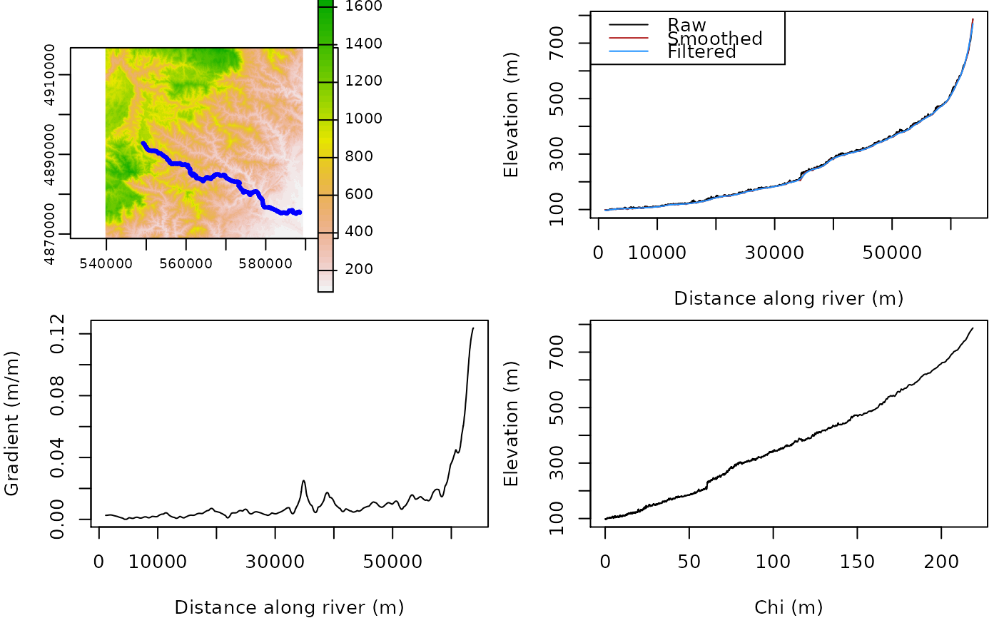
# get river data
# see DEM processing vignette for example of the extraction of such data from a DEM
data("rivers_cevennes",package = "gtbox")

# get DEM (for plotting)
data("dem_cevennes",package = "gtbox")
dem = rast(dem_cevennes)
rm(dem_cevennes)

df = rivers_cevennes[rivers_cevennes$river==1,] # select a river
df = df[order(df$dist),] # order data according to distance along river
df$area = df$acc*30^2 # compute drainage area
df$chi = profile_chi(df$area,df$dist,aref=1000,mn=0.5) # compute chi
df$z2 = profile_smooth(df$dist,df$z,span=0.1,radius=10e3) # smooth profile
df$z3 = profile_gaussian(df$dist,df$z2,span=0.1,sigma=500) # filter profile
df$gradient = profile_gradient(df$dist,df$z3,window=200) # compute gradient

par(mfrow=c(2,2))
plot(dem)
lines(df$x,df$y,lwd=3,col="blue")
par(mar = c(4,4,0.5,0.5))
plot(df$dist,df$z,type="l",xlab="Distance along river (m)",ylab="Elevation (m)")
lines(df$dist,df$z2,col="firebrick")
lines(df$dist,df$z3,col="dodgerblue")
legend("topleft",c("Raw","Smoothed","Filtered"),lty=1,col=c("black","firebrick","dodgerblue"))
plot(df$dist,df$gradient,type="l",xlab="Distance along river (m)",ylab="Gradient (m/m)")
plot(df$chi,df$z,type="l",xlab="Chi (m)",ylab="Elevation (m)")